This is an introduction to NumPyro, using the Eight Schools model as example.
Here we demonstrate the effects of model reparameterisation. Reparameterisation is especially important in hierarchical models, where the joint density tend to have high curvatures.
| |
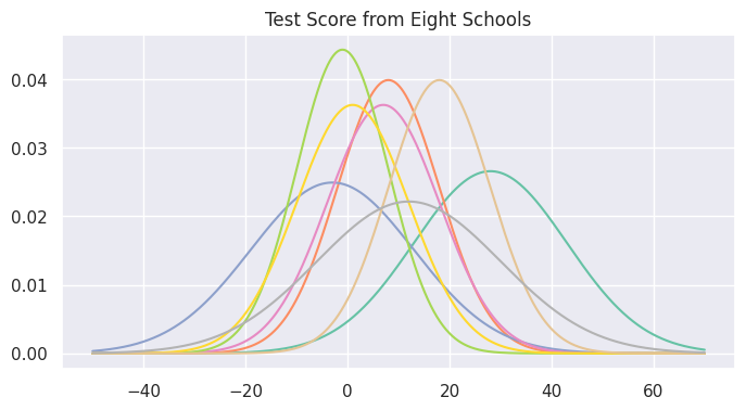
Here we are using the classic eight schools dataset from Gelman et al. We have collected the test score statistics for eight schools, including the mean and standard error. The goal, is to determine whether some schools have done better than others. Note that since we are working with the mean and standard error of eight different schools, we are actually modeling the statistical analysis resutls of some other people: this is essentially a meta analysis problem.
| |
Visualize the data.
| |
The baseline model
The model we are building is a standard hierarchical model. We assume that the observed school means represent their true mean \(\theta_n\), but corrupted with some Normal noise, and the true means are themselves drawn from another district level distribution, with mean \(\mu\) and standard deviation \(\tau\), which are also modeled with suitable distributions. Essentially it’s Gaussian all the way up, and we have three different levels to consider: student, school, and the whole district level population.
\begin{align*} y_n &\sim \text{N} (\theta_n, \sigma_n) \\ \theta_n &\sim \text{N} (\mu, \tau) \\ \mu &\sim \text{N} (0, 5) \\ \tau &\sim \text{HalfCauchy} (5). \end{align*}
In NumPyro models are coded as functions.
| |
Note that the code and the mathematical model are almost identical, except that they go in different directions. In the mathematical model, we start with the observed data, and reason backward to determine how they might be generated. In the code we start with the hyperparameters, and move forward to generate the observed data.
J and sigma are data we used to build our model, but they are not
part of the model, in the sense that they are not assigned any
probability distribution. y, on the other hand, is the central
variable of the model, and is named obs in the model.
numpyro.plate is used to denote that the variables inside the plate
are conditionally independent. Probability distributions are the
building blocks of Bayesian models, and NumPyro has a lot of them. In
NunPyro, probability distributions are wrappers of JAX random number
generators, and they are translated into sampling statements using the
numpyro.sample primitive.
However numpyro.sample is used to define the model, not to draw
samples from the distribution. To actually draw samples from a
distribution, we use numpyro.infer.Predictive. In numpyro each model
defines a joint distribution, and since it’s a probability distribution,
we can draw samples from it. And since we haven’t conditioned on any
data, the samples we draw are from the prior distribution.
Sampling directly from the prior distribution, and inspect the samples, is a good way to check if the model is correctly defined.
| |
| |
When the samples of some variables are observed, we can condition on
these observations, and infer the conditional distributions of the other
variables. This process is called inference, and is commonly done using
MCMC methods. The conditioning is done using the
numpyro.handlers.condition primitive, by feeding it a data dict and
the model.
Since we have a GPU available, we will also configure the MCMC sampler to use vectorized chains.
| |
| |
The NUTS sampler is a variant of the Hamiltonian Monte Carlo (HMC) sampler, which is a powerful tool for sampling from complex probability distributions. HMC also comes with its own set of diagnostics, which can be used to check the convergence of the Markov Chain. The most important ones are the effective sample size and the Gelman-Rubin statistic, which is a measure of the convergence of the Markov Chain.
| |
| |
The effective sample size for \(\tau\) is low, and judging from the
r_hat value, the Markov Chain might not have converged. Also, the
large number of divergences is a sign that the model might not be well
specified. Here we are looking at a prominent problem in hierarchical
modeling, known as Radford’s funnel, where the posterior distribution
has a very sharp peak at the center, and a long tail, and the curvature
of the distribution is very high. This seriously hinders the performance
of HMC, and the divergences are a sign that the sampler is having
trouble exploring the space.
However, the issue can be readily rectified using a non-centered parameterization.
Manual reparameterisation
The remedy we are proposing is quite simple: replacing
\[ \theta_n \sim \text{N} (\mu, \tau) \]
with
\begin{align*} \theta_n &= \mu + \tau \theta_0 \\ \theta_0 &\sim \text{N} (0, 1). \end{align*}
In essence, instead of drawing from a Normal distribution whose parameters are themselves variables in the model, we draw from the unit Normal distribution, and transform it to get the variable we want. By doing so we untangled the sampling process of \(\theta\) from that of \(\mu\) and \(\tau\).
| |
Here we use another primitive, numpyro.deterministic, to register the
transformed variable, so that its values can be stored and used later.
| |
| |
we can see the mean and variance are indeed quite close to that of the unit normal.
Condition on the observed data and do inference.
| |
| |
This looks much better, both the effective sample size and the r_hat
have massively improved for the hyperparameter tau, and the number of
divergences is also much lower. However, the fact that there are still
divergences tells us that reparameterisation might improve the topology
of the posterior parameter space, but there is no guarantee that it will
completely eliminate the problem. When doing Bayesian inference,
especially with models of complex dependency relationships as in
hierarchical models, good techniques are never a sufficient replacement
for good thinking.
Using numpyro’s reparameterisation handler
Since this reparameterisation is so widely used, it has already been implemented in NumPyro. And since reparameterisation in general is so important in probabilistic modelling, NumPyro has implemented a wide suite of them.
In probabilistic modeling, although it’s always a good practice to
separate modeling from inference, it’s not always easy to do so. As we
have seen, how we formulate the model can have a significant impact on
the inference performance. When building the model, not only do we need
to configure the variable transformations, but we also need to inform
the inference engine how to handle these transformed variables. This is
where the numpyro.handlers.reparam handler comes in.
| |
The process of reparameterisation goes as follows:
- Start with a standard Normal distribution
dist.Normal(0., 1.), - Transform it using the affine transformation
AffineTransform(mu, tau), - Denote the result as a
TransformedDistribution, - Register the transformed variable
thetausingnumpyro.sample, - Inform the inference engine of the reparameterisation using
reparam.
Proceed with prior predictive sampling.
| |
| |
Condition on the observed data and do inference.
| |
| |
The model reparameterised using handlers, as we can see, performs just like the manually reparameterised one, with the same mean and variance estimation, same effective number of samples, and the same number of divergences.
The results are consistent with the manual reparameterisation. It might seem uncessarily complicated to use the reparameterisation handler in this simple example, but in more complex models, especially those with many layers of dependencies, the reparameterisation handler can greatly facilitate the model building process.