9 Regularisation

9.1 Inductive bias

Inductive bias refers to the set of assumptions a model makes about the patterns it expects to find in the data. These biases help the model to generalize better from the training data to unseen instances, guiding the learning process towards more plausible solutions given limited information. In the context of deep learning, inductive bias can be inherent in the architecture of the network, the choice of optimization algorithm, or the data representation itself.

9.1.1 Inverse problem

In the Bayesian sense, the forward problem is sampling, the inverse problem is inference. data –> parameter

9.1.2 No free lunch theorem

Since there is no universally best learner for every task, the success of a learning algorithm on a particular task depends on how well its inductive bias aligns with the problem.

Regularization methods contribute to an algorithm’s inductive bias, thus affecting its performance across different tasks.

models are essentially a set of assumptions, and assumptions have consequences

9.1.3 Symmetry and invariance

9.1.4 Equivariance

9.2 Weight decay

smaller weights, simpler models L2 regularisation

9.2.1 Consistent regularizers

9.2.2 Generalised weight decay

9.3 Learning curves

On the modeling side, there can be several different approaches to increase the generalization performance:

increase the model size (better representative capability);
increase the data size (capturing more pattern and less noise);
regulariation (through weight-decay or other methods);
improve the model architecture (inducing more inductive bias for certain problems);
model averaging (reduce the variance in specific models)

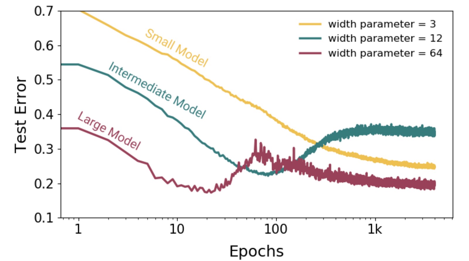
Another factor that influences the bias-variance trade-off is the learning process itself. During optimization of the error function through gradient descent, the training error typically decreases as the model parameters are updated, whereas the error for hold-out data may be non-monotonic. This behaviour can be visualized using learning curves, which plot performance measures such as training set and validation set error as a function of iteration number during an iterative learning process such as stochastic gradient descent. These curves provide insight into the progress of training and also offer a practical methodology for controlling the effective model complexity.

9.3.1 Early stopping

9.3.2 Double descent

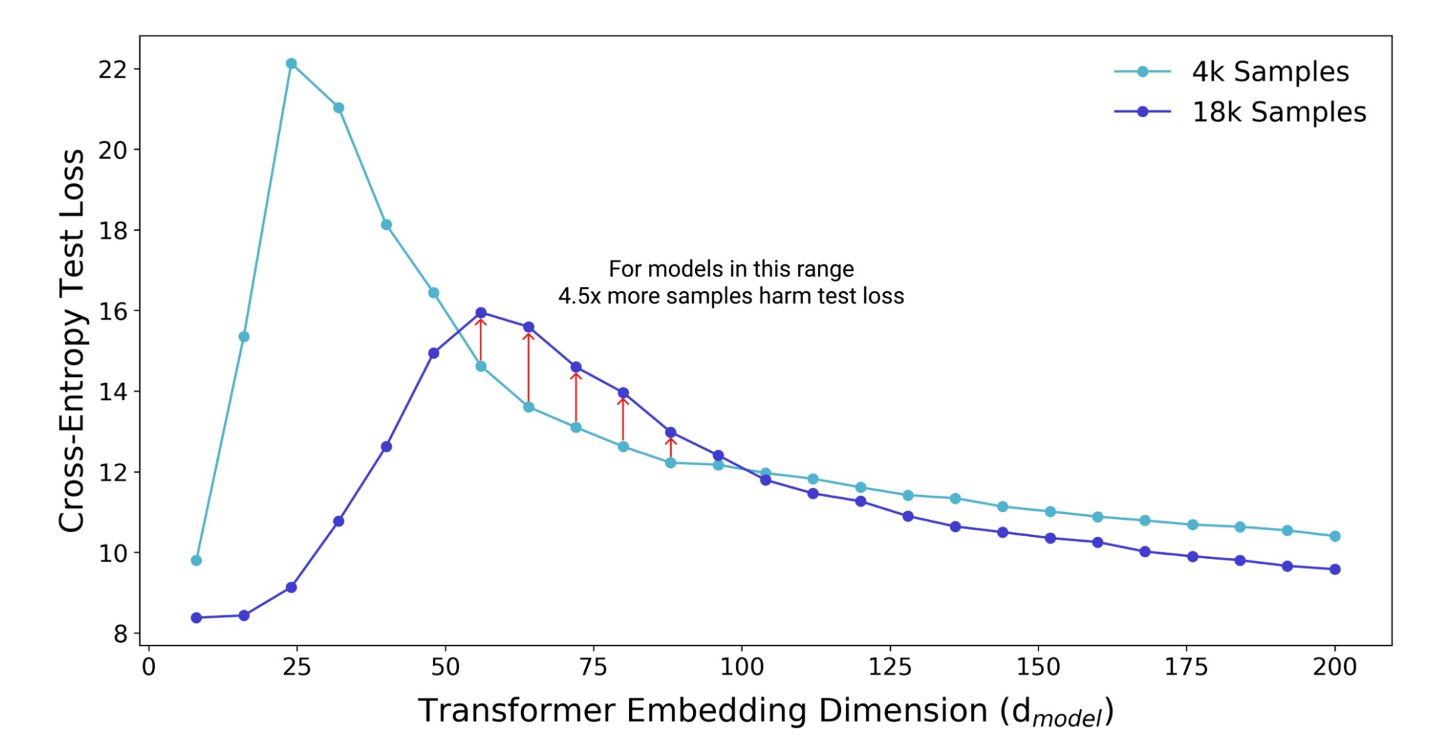
Double descent entends the bias-variance trade-off to the big-data/large-model regime where we have so much data that we can fit a model of any size to it.

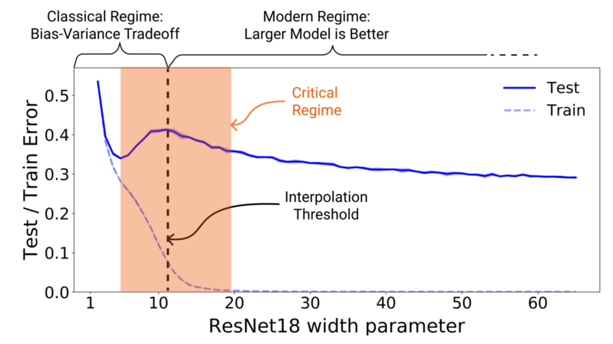
In the classical regime, we have limited data, thus we seek a bias-variance balance. In the modern regime, since we have so much data, increasing the model size always leads to better test results.

The black dashed line marks the interpolation threshold, where the model’s capacity is just enough to perfectly fit the training data.

stochastic gradient descent not only makes the training more feasible, but also makes the model more robust.

9.5 Residual connections

9.6 Model averaging

9.6.1 Dropout

Randomly “dropping out” a subset of neurons or connections during training encourages the network to develop redundant representations and prevents co-adaptation of features. The inductive bias here is towards models that are robust to the loss of individual pieces of information, reflecting a kind of ensemble learning within a single model.